
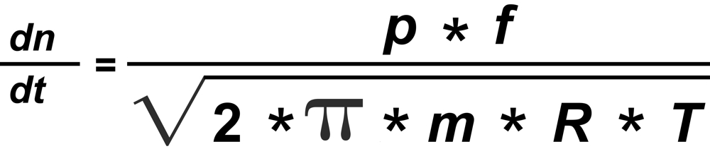
"s" is the sensitivity (e.g. in [Asec/mol])
And finally:
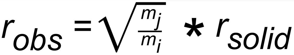
Note: We assume the sensitivity for two isotopic species of the same element as being equal
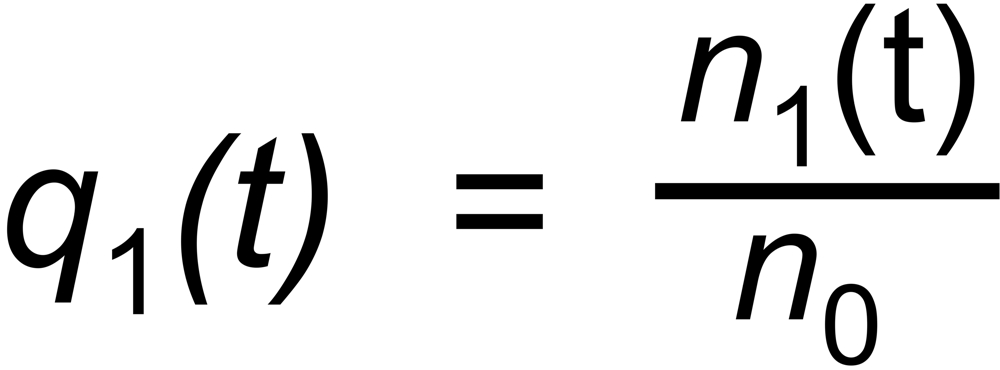
Let us assume that we have loaded n1 resp. n2 moles of two isotopic species (1,2), i.e. a total of n = n1 + n2 moles.
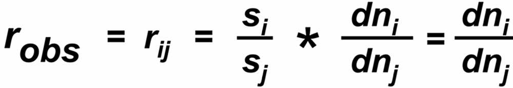
The 'observed isotope ratio', i.e. the ratio of the two relevant ion currents is, therefore, given by
"f" is the mol fraction, "m" the mass and "p" the vapor pressure of the particular isotopic species.
From Langmuir's Law we know the rate of evaporation from a solid surface
Note: The ratio of the mol fractions is the isotope ratio in the yet solid phase of the sample, which can be computed, using Rayleigh's law.
Their masses are m1 < m2 < m3, i.e., in our example,both ratios always have one species with the same mass in common (m1, m2, or m3).
(For details, see K.Habfast, Int. J. Mass. Spectrom. 89 (1983) p. 165)
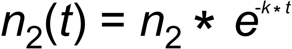
Let us, as an example, assume that the number dn2(t) of moles of species (2), evaporating per unit time from the filament at time t , is proportional to the number of moles n2(t), present on the filament. This, eventually, results in an exponential decay of the amount of this species (and, as a consequence, of its ion current):
Let us, as an example, assume that the number dn2(t) of moles of species (2), evaporating per unit time from the filament at time t , is proportional to the number of moles n2(t), present on the filament. This, eventually, results in an exponential decay of the amount of this species (and, as a consequence, of its ion current):
The strict application of these equations , hence, sets some restrictions for the definition of the
involved ratios and requires different algorithms for the four legal ratio definitions.
Such restrictions can be circumvented by the application of the third Rayleigh equation, which
relates fractionation to the total amount of sample on the filament. However, the elimination of the
mol fraction q does not result in an exlicite expression for RT. Therefore, RT must be calculated
by the application of, either, the 'regula falsi (secant method)' , or, of 'Newton's algorithm (tangent
method)'.
Both algorithms normally converge within a few iteration loops (less than 10), except for very
noisy data, which may cause difficulties.
In such cases, one better switches to one of the empiric fractionation laws, which are described
in the following. (If the iteration does not converge, your data are, for sure, so noisy that virtually
any systematic error of the computed result cannot be pushed over to the particular fractionation
correction algorithm).
If the lower masses of the known and the unknown ratios are equal, the non-iterative equation
delivers the accurate Rayleigh normalization value.
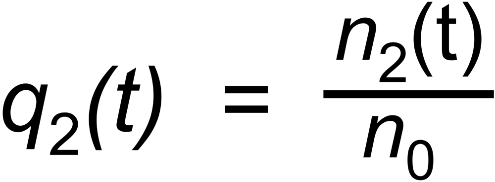
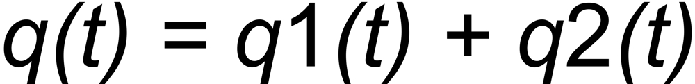
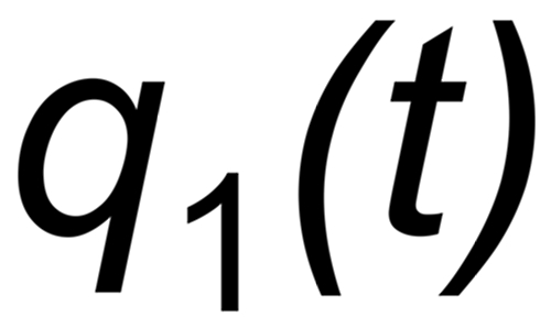
Let be
the (time dependent) mole fractions of these species and
and
the mole fraction of the whole sample on the filament.
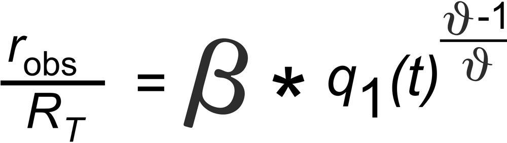
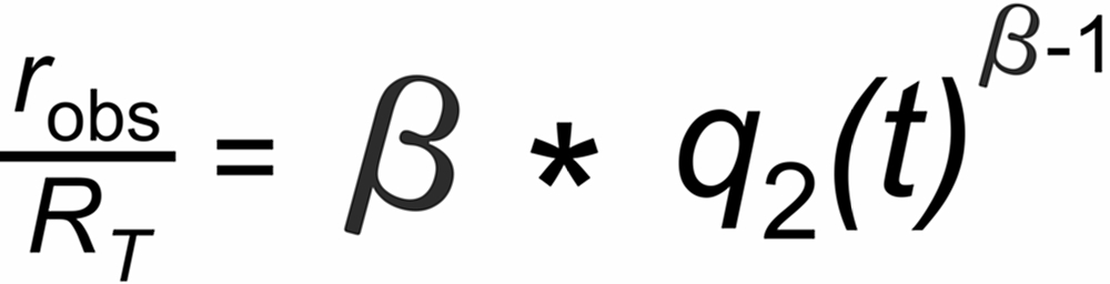
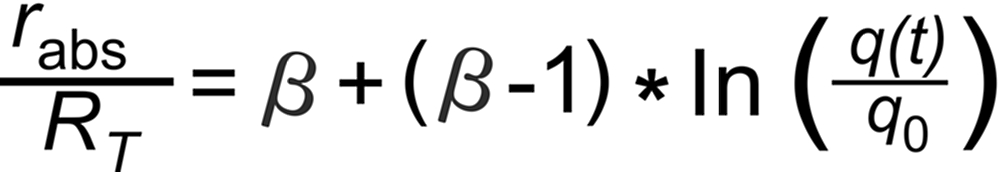
Then, the Rayleigh Law describes the time dependence of the measured ratio (rabs) as follows (see footnote 1):
or
or
During a thermal ionization (TIMS) isotope ratio measurement, everybody can easily observe, that isotope ratios systematically vary with time. This effect is called fractionation.
It has a simple reason: For the lighter isotopic species of an isotope ratio, the rate of evaporation is higher than for the heavier species. Hence, the lighter isotope is depleted with time in the not yet evaporated fraction of the sample. And, vica versa, it is, at any time, enriched in the vapor phase, as compared to the remaining solid phase.
Thus, in order to describe fractionation mathematically, it suggests itself, to relate fractionation and sample consumption. This is what the Lord Rayleigh's 'law' (1896) does: It describes the time dependence of the isotope ratio in the not yet evaporated fraction of the sample.
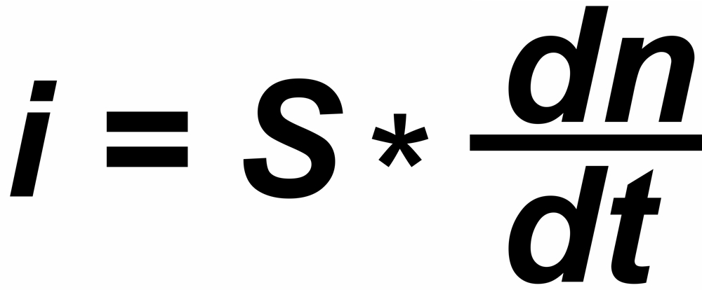
In a thermal ionization source, the ion current 'i' reflects the rate of flow (dn/dt) of those particals which hit the hot surface.
It has a simple reason: For the lighter isotopic species of an isotope ratio, the rate of evaporation is higher than for the heavier species. Hence, the lighter isotope is depleted with time in the not yet evaporated fraction of the sample. And, vica versa, it is, at any time, enriched in the vapor phase, as compared to the remaining solid phase.
Thus, in order to describe fractionation mathematically, it suggests itself, to relate fractionation and sample consumption. This is what the Lord Rayleigh's 'law' (1896) does: It describes the time dependence of the isotope ratio in the not yet evaporated fraction of the sample.
In a thermal ionization source, the ion current 'i' reflects the rate of flow (dn/dt) of those particals which hit the hot surface.
Inserting n2(t)/n2 into the linearized approximation results in
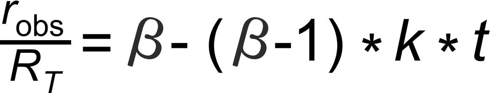
RT is the true isotope ratio.
A very good (linearized) approximation of this law is given by
A very good (linearized) approximation of this law is given by
Hence, we may expect roughly linear decay (or increase, if b<1 ) of the fractionation pattern with time for an exponentially decaying ion current.
Other than exponential emission profiles produce other, sometimes strange, fractionation patterns. Oftenly, the fractionation pattern also reflects a particular evaporation behaviour, like varying multiple species emission and so on.
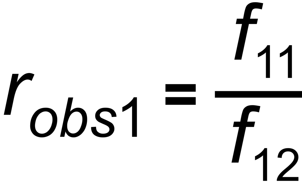
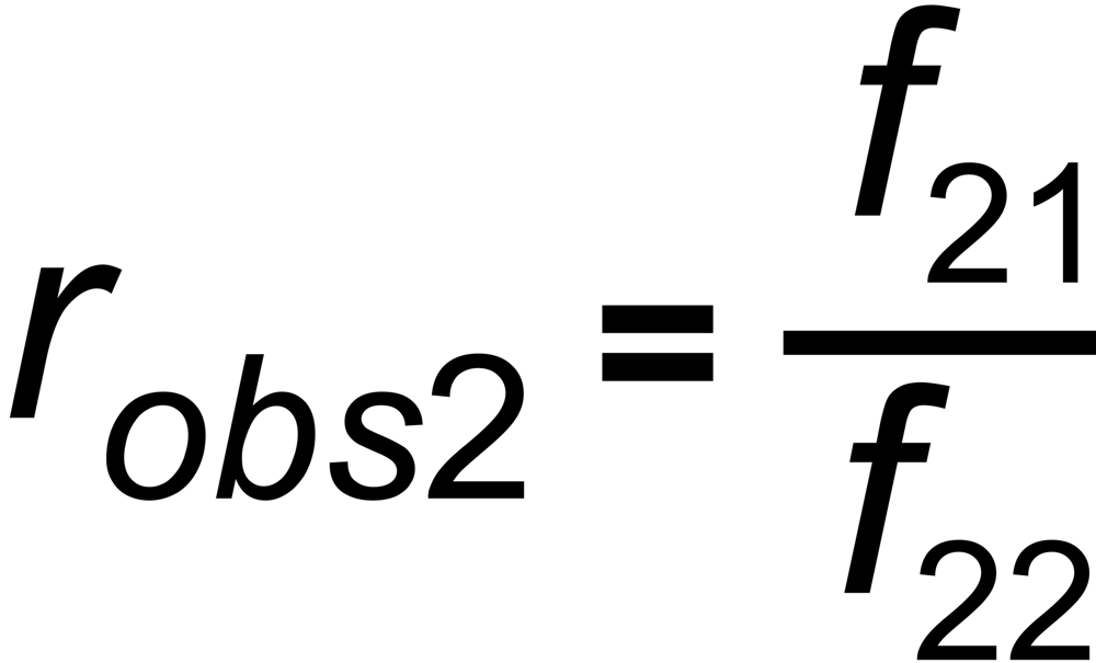
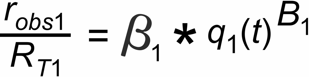
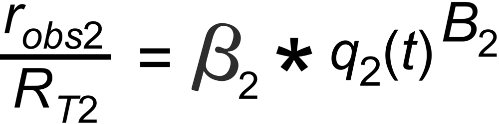
Let us now consider the Rayleigh equations of two isotope ratios (e.g. the unknown and the known ratio in a three isotope system).
Other than exponential emission profiles produce other, sometimes strange, fractionation patterns. Oftenly, the fractionation pattern also reflects a particular evaporation behaviour, like varying multiple species emission and so on.
Let us now consider the Rayleigh equations of two isotope ratios (e.g. the unknown and the known ratio in a three isotope system).
and
;
Let be
the mole fraction of this species. We thus get two equations
and
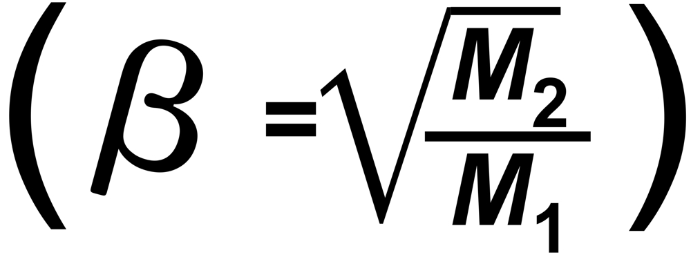
with
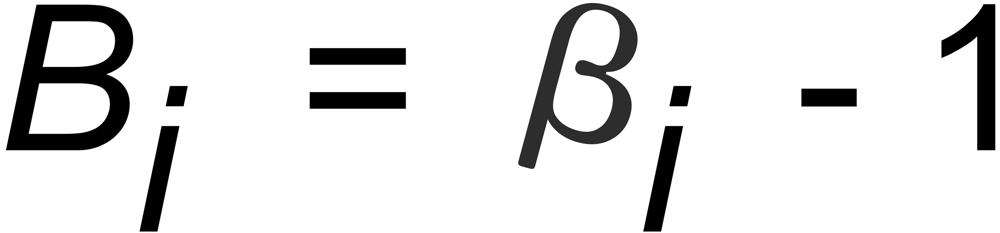
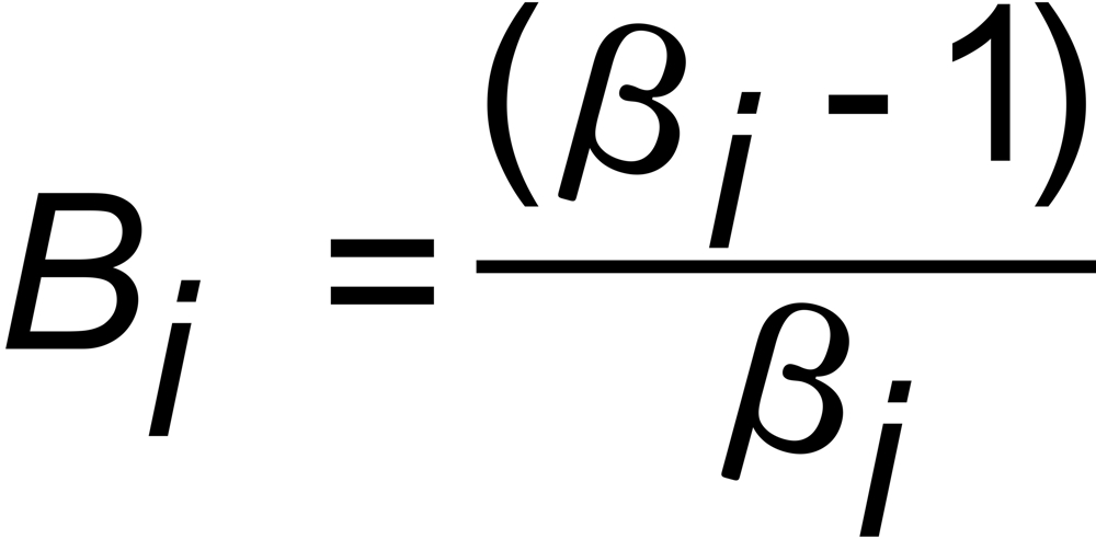
and
(i=1,2)
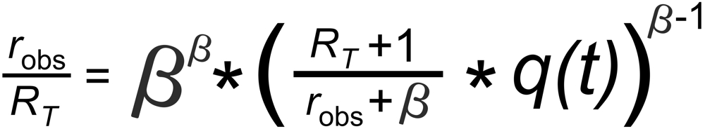
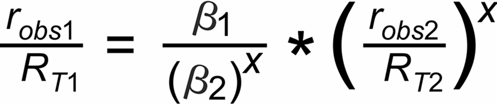
If q(t) is assigned to the same species in both ratios, the above equations can be combined for elminating q(t):
This above equation describes a relation, which is called 'fractionation line' in its graphical representation.
In its numeric version, it is used to calculate the true isotope ratio RT1 , given the measured ratios robs1 and robs2, and the true ratio RT2 of the internal reference.
For the assignment of the common species in the two relevant ratios we appearantly have to distinguish between 4 cases (given that both ratios are defined with either the light or the heavy species in the nominator, respectively):
(A): m1 is common to both ratios,
(B): m2 is in the nominator of r1 and in the denominator of r2,
(C): m2 is in the denominator of r1 and in the nominator of r2,
(D): m3 is common to both ratios.
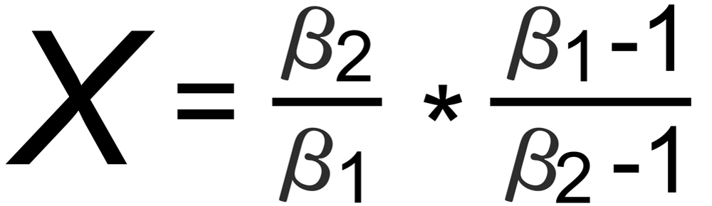
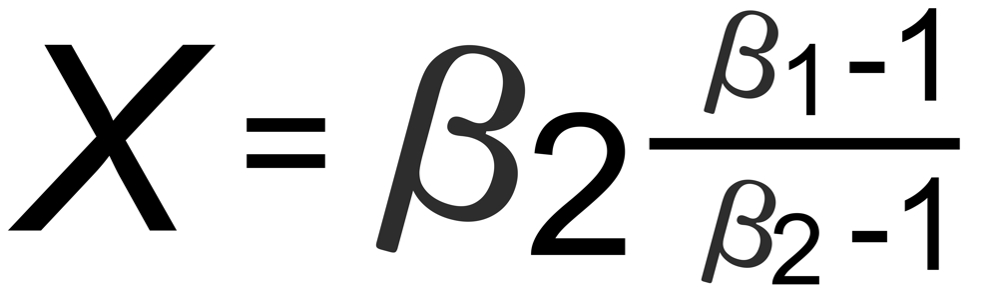
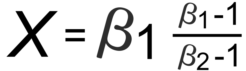
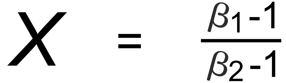
Hence, the exponent X in the above equation is, respectively, given by:
In its numeric version, it is used to calculate the true isotope ratio RT1 , given the measured ratios robs1 and robs2, and the true ratio RT2 of the internal reference.
For the assignment of the common species in the two relevant ratios we appearantly have to distinguish between 4 cases (given that both ratios are defined with either the light or the heavy species in the nominator, respectively):
(A): m1 is common to both ratios,
(B): m2 is in the nominator of r1 and in the denominator of r2,
(C): m2 is in the denominator of r1 and in the nominator of r2,
(D): m3 is common to both ratios.
Hence, the exponent X in the above equation is, respectively, given by:
A
B
C
D


Dr. Karleugen Habfast: Theory of Fractionation Correction - Introduction


